How to classify ICA components
About this guide
This post explains how to classify noise and signal components obtained from single-subject ICA. These hand-labelled components can be later used for ICA-based cleaning of fMRI data. I focus here on the practical steps rather than the theoretical background. For a deeper dive into the methods and the tools used here, check out the resources linked at the end. For ICA-based noise removal, have a look at this post.
Background
In resting-state fMRI processing, we often apply Independent Component Analysis (ICA) to split the data into components, either to clean the data of structured noise or to analyse the signal components we find. In either case, we need to identify which components are noise-driven and which are dominated by signal.
ICA is a dimensionality reduction method, similar to Principal Component Analysis (PCA). That means, ICA reduces the high-dimensional raw functional data into a low-dimensional representation. Put differently, ICA finds patterns in the data that are independent form each other and explain substantial variance in the data. By breaking down the data into these patterns, or components, ICA separates the data into components that reflect BOLD signal and components that reflect noise (physiological, imaging reconstruction artefacts, movement, etc.).
ICA components consist of a single 3D spatial maps and an associated time course. Using the map, the timecourse and a frequency domain representation of the timecourse, we can identify the noise components, label them, and regress their associated variance out of the raw data - thereby removing the noise.
Classifying components
How do I recognize noise and signal components?
In order to separate noise from signal, we need to look at the spatial map, timecourse and power spectrum and judge whether this reflects more signal or more noise. In general, we don’t want to throw away any signal, so when in doubt we leave components in the data by labelling the components as Unknown. Innoncent until proven guilty is the mantra.
The best way to learn how to recognize noise components in your own data is to look at them. Pull up the melodic_IC.nii.gz file of an example subject from your dataset and click through the components.
fsleyes --scene melodic -ad subject-01/run-01.feat/filtered_func_data.ica
I also like to open the plots of the motion parameters generated automatically by the FEAT report. FEAT only generates these if you have run motion correction within FEAT. For that, run open subject-01/run-01.feat/report_prestats.html or point your browser at the report_prestats.html file. This is very useful to compare the timecourse of the component you are looking at with the motion parameters. Sometimes you can spot a movement noise component by their exact match with one of the motion parameter timecourses.
If you have not run motion correction within FEAT, but, say, with SPM, you can generate those plots quickly with fsl_tsplot. The SPM-output text file starting with rp_ contains the movement parameters of the scan as estimated during SPM motion correction. The file contains six columns. These represent position (not movement) of the subject in terms of X, Y, and Z displacement and X, Y, and Z axis rotation with respect to the first scan entered. The first three columns are in millimeters and the last three are in degrees. Run the following to generate and open the motion parameter plots:
fsl_tsplot -i subject-01/run-01.feat/rp_run_01.txt -t 'SPM estimated rotations (radians)' -u 1 --start=1 --finish=3 -a x,y,z -w 800 -h 300 -o subject-01/run-01.feat/rot_01.png
fsl_tsplot -i subject-01/run-01.feat/rp_run_01.txt -t 'SPM estimated translations (mm)' -u 1 --start=4 --finish=6 -a x,y,z -w 800 -h 300 -o subject-01/run-01.feat/trans_01.png
fsl_tsplot -i subject-01/run-01.feat/rp_run_01.txt -t 'SPM estimated rotations and translations (mm)' -u 1 --start=1 --finish=6 -a "x(rot),y(rot),z(rot),x(trans),y(trans),z(trans)" -w 800 -h 300 -o subject-01/run-01.feat/rot_trans_01.png
open subject-01/run-01.feat/*_01.png
This should pull up plots like this where you can see the movements (in this case translations in mm) over time:
![]()
By comparing the timecourse of the components for this scan with the movement parameters over time, you can identify noise components that are dominated by movement.
Higher quality datasets
In some datasets, noise and signal will be easier to recognize than in others. In high quality datasets, labelling is usually easier than in datasets of lower quality. Nevertheless, noise shares some features that are recognizable in dataset of all kinds. I will walk through some examples here, starting with high quality data to get a feel for what clearly distinguishable noise and signal looks like. The resting-state scans in this dataset consist of many timepoints (~600 volumes), have a low TR (1 second) and a relatively small voxel size (2.5 x 2.5 x 3 mm).
Signal
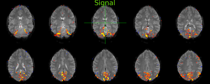
Look at the component below. The spatial map of the component shows signal stemming mostly form voxels within the brain, that look like they are confined to grey matter (little contribution from white matter and ventricular voxels). It also looks like biologically plausible signal, since it appears spatially contiguous. Examine the time series plot in the bottom left corner and the Power spectrum in the bottom right corner shown in fsleyes. The component is easily identifiable as signal from its smooth, BOLD-like timecourse (bottom left) that has most of its power at low frequencies below 0.1 Hz (bottom right). Generally, BOLD signal will have its highest power between 0.01 and 0.1 Hz, although higher frequencies can occur.
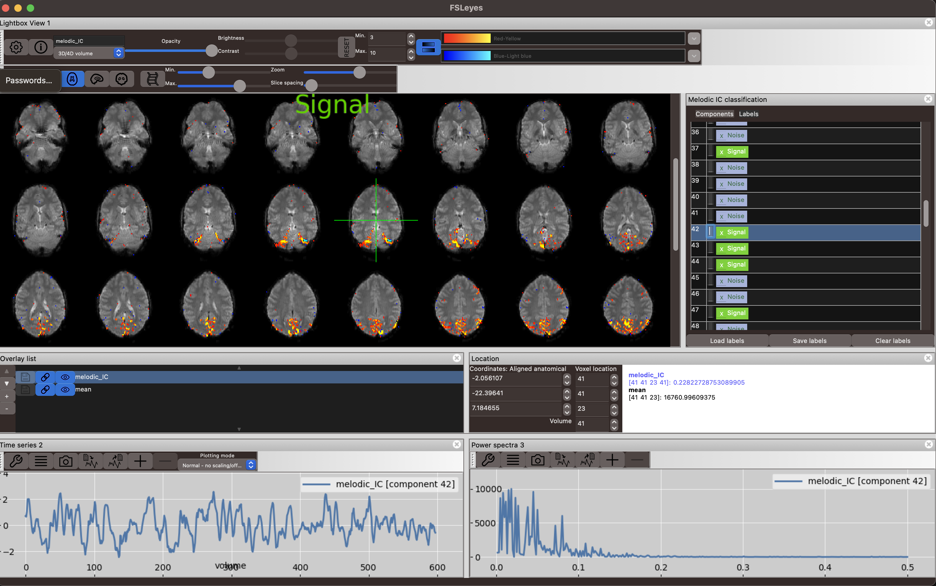
The same goes for the second signal component. Signal is coming primarily from grey matter voxels, that seems biologically plausible, as it appears uninterrupted in several axial slices and contiguous lines that follow a gyral pattern. The timecourse looks smooth and the power spectrum shows high power in the lower frequency range below 0.1 Hz.
Noise
Now let’s look at a few noise components. These will usually appear as the earliest components in the data, so they will explain the most variance. It often can take 10-20 components of noise until the first signal component pops up, so don’t be surprised if you have to click through quite a few noise components until hitting some signal! In fact, more than 70% of components will be noise, so don’t worry if most of what you can find will be noise. The data can still have a lot of signal in it, the noise components simply outnumber it. But this goes to show how important thorough is for resting-state data.
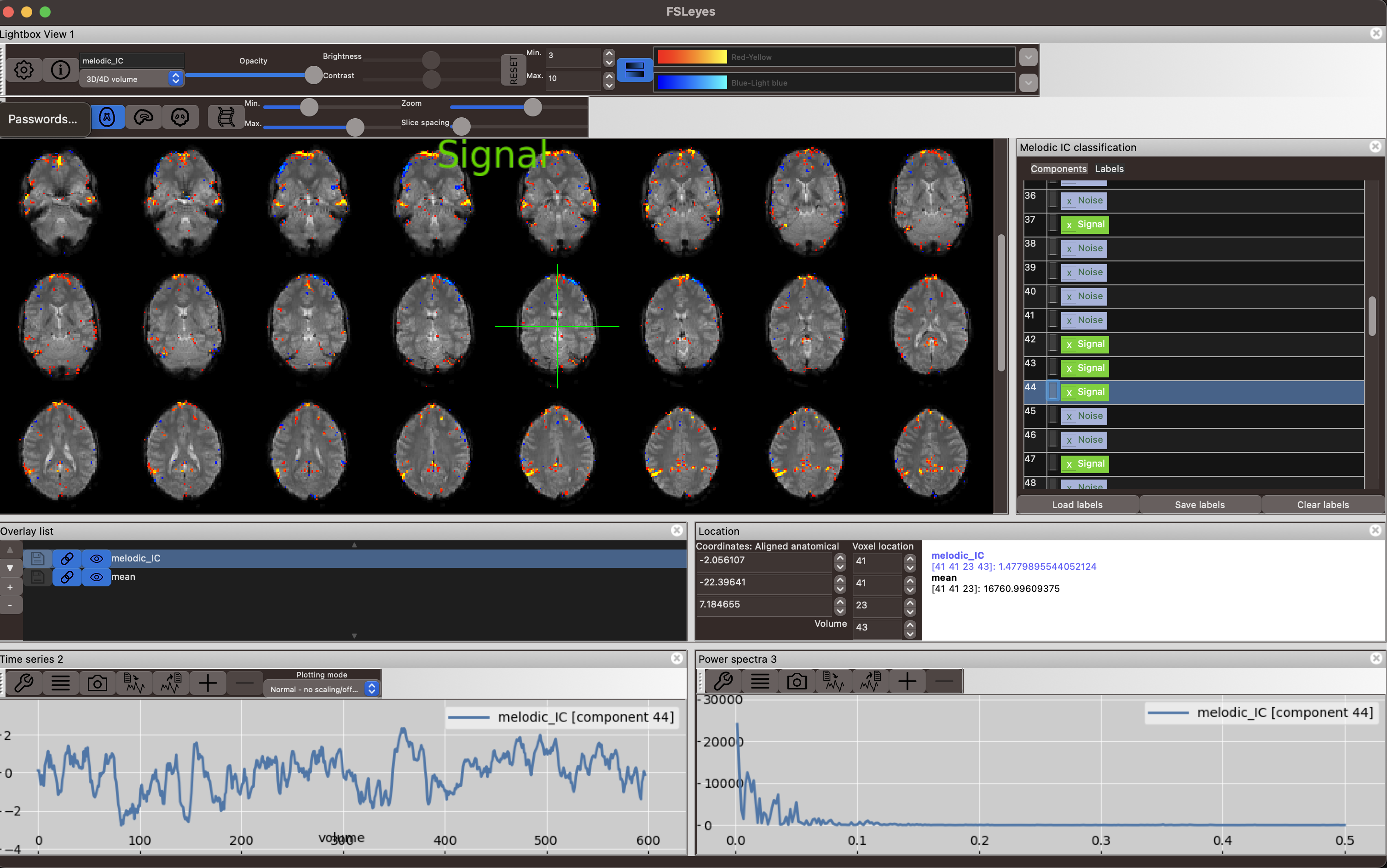
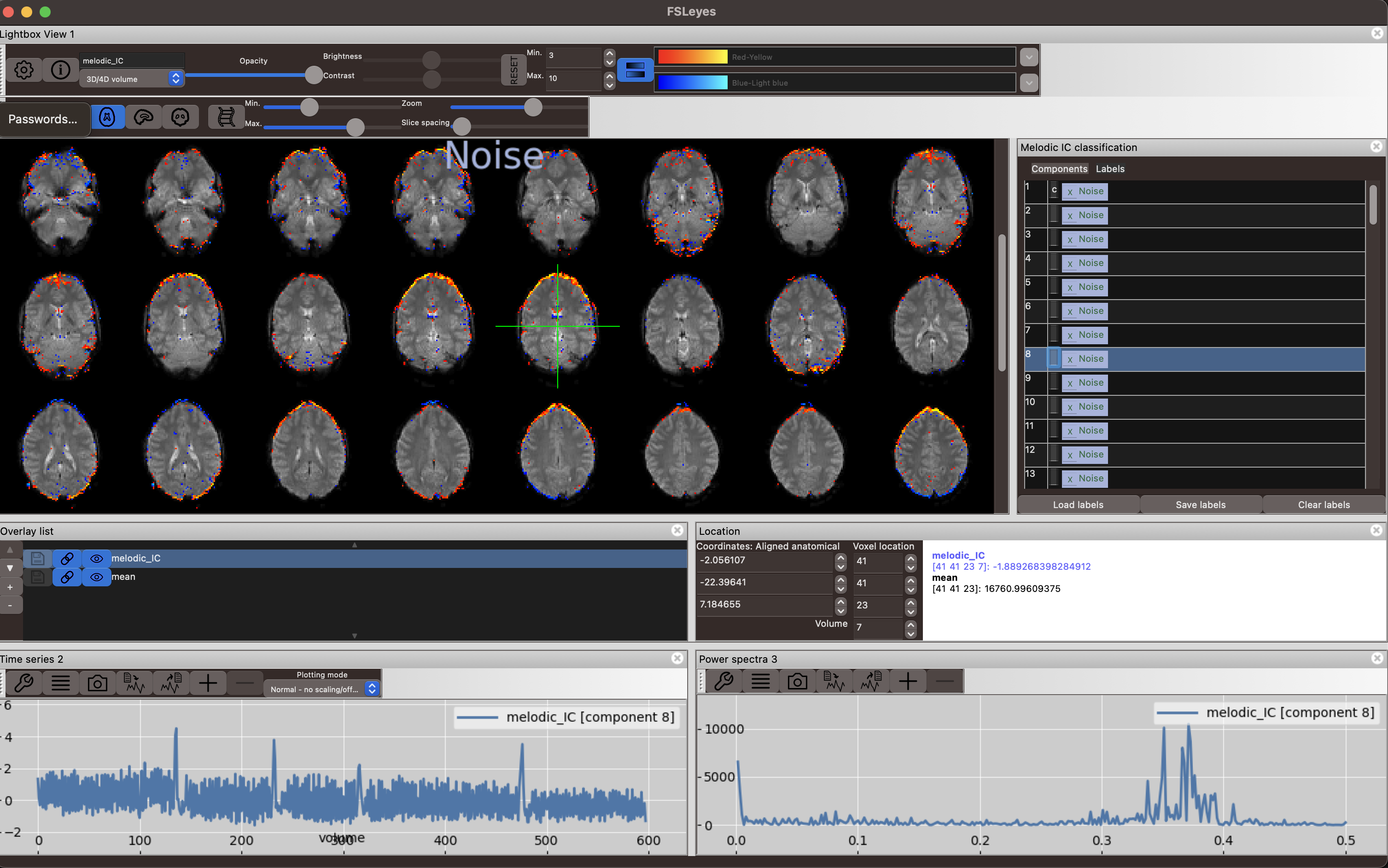
Below you can see a clear noise component. The strongest contributions to this component are made by voxels that are clearly outside of the brain and the timecourse shows sharp jumps. This component likely comes from a sudden head movement at around volume 490.
Another noise component in the figure below shows very high frequency fluctuations as seen in the power spectrum and the time series plot. The spatial map shows a ringing around the brain that does not seem confined to gyri inside the brain.
Lower quality datasets
The data in the next dataset we will look at is of relatively lower quality, with fewer volumes acquired (only 100), slightly larger voxels (3 x 3 x 3 mm) and from a patient population that is prone to moving in the scanner. Still, we can still distinguish some of the noise and signal components clearly in the data.
Signal
This signal component shows high activity in the grey matter and little to no contributions from voxels outside the brain or in white matter and ventricles Although the smoothness of the timecourse is less pronounced in this signal components because fewer volumes were acquired in this data, it still shows the low frequency fluctuations we would expect from BOLD signal. The power spectrum peaks at around 0.1 Hz, as expected.
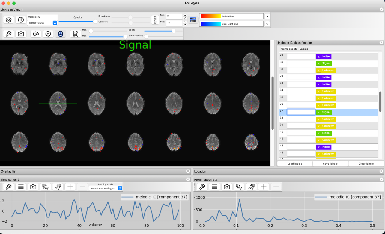
Spatial map, slow timecourse and the low frequency power spectrum identify this component as signal as well.
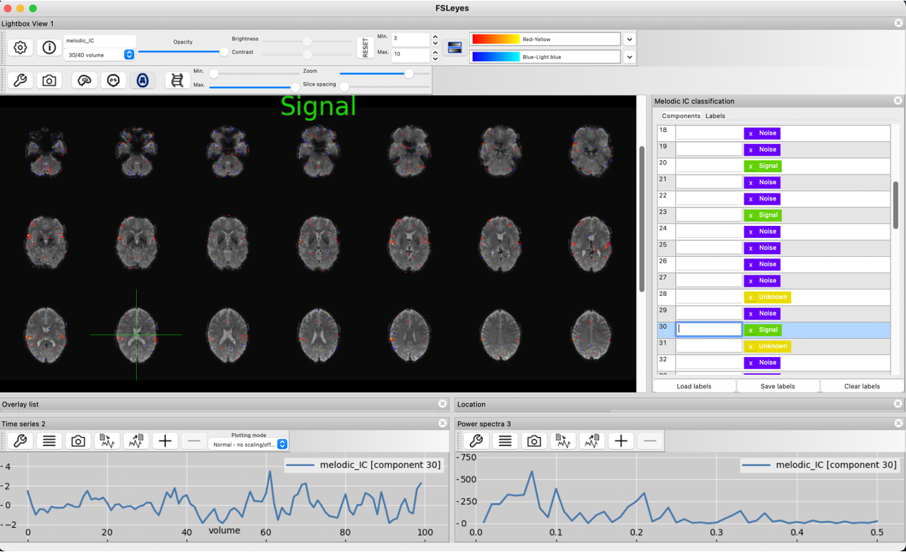
This component also shows the characteristic contributions from voxels in grey matter that are spatially contiguous, show a smooth timecourse and a low power spectrum of BOLD signal.
Noise
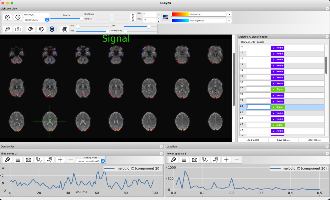
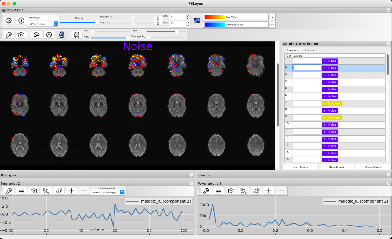
Here, we can see the spatial map clearly indicates noise by the brightest voxels located outside of the brain in areas that suffer from signal dropout. This noise is likely induced by susceptibility artefacts. Due to the few volumes, the timecourse appears less characteristically noisy than we saw in the noise components of the high quality dataset. Nonetheless, the spatial map is a clear sign that this component is dominated by noise.
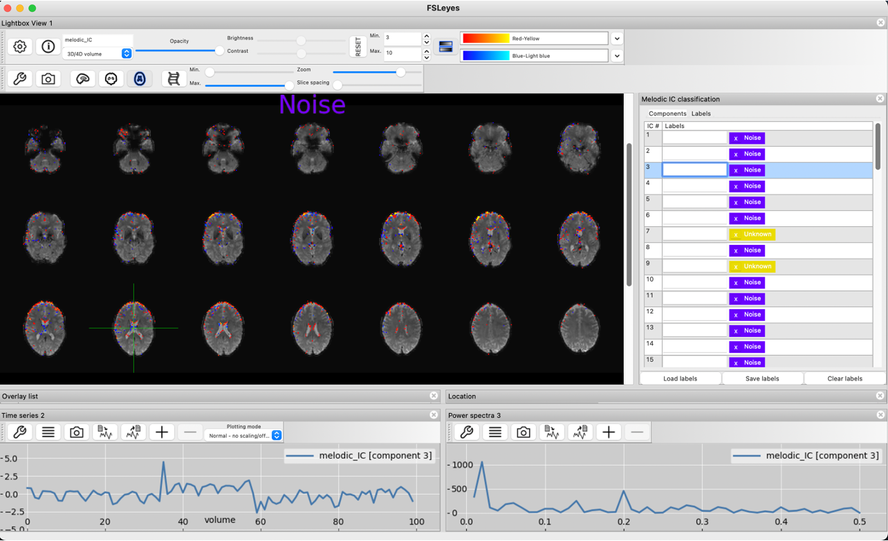
The typical ringing around the front of the brain identifies this component as noise. Moreover, the high contributions from voxels within the ventricles and the jumps in the timecourse confirm that this component should be classified as noise.
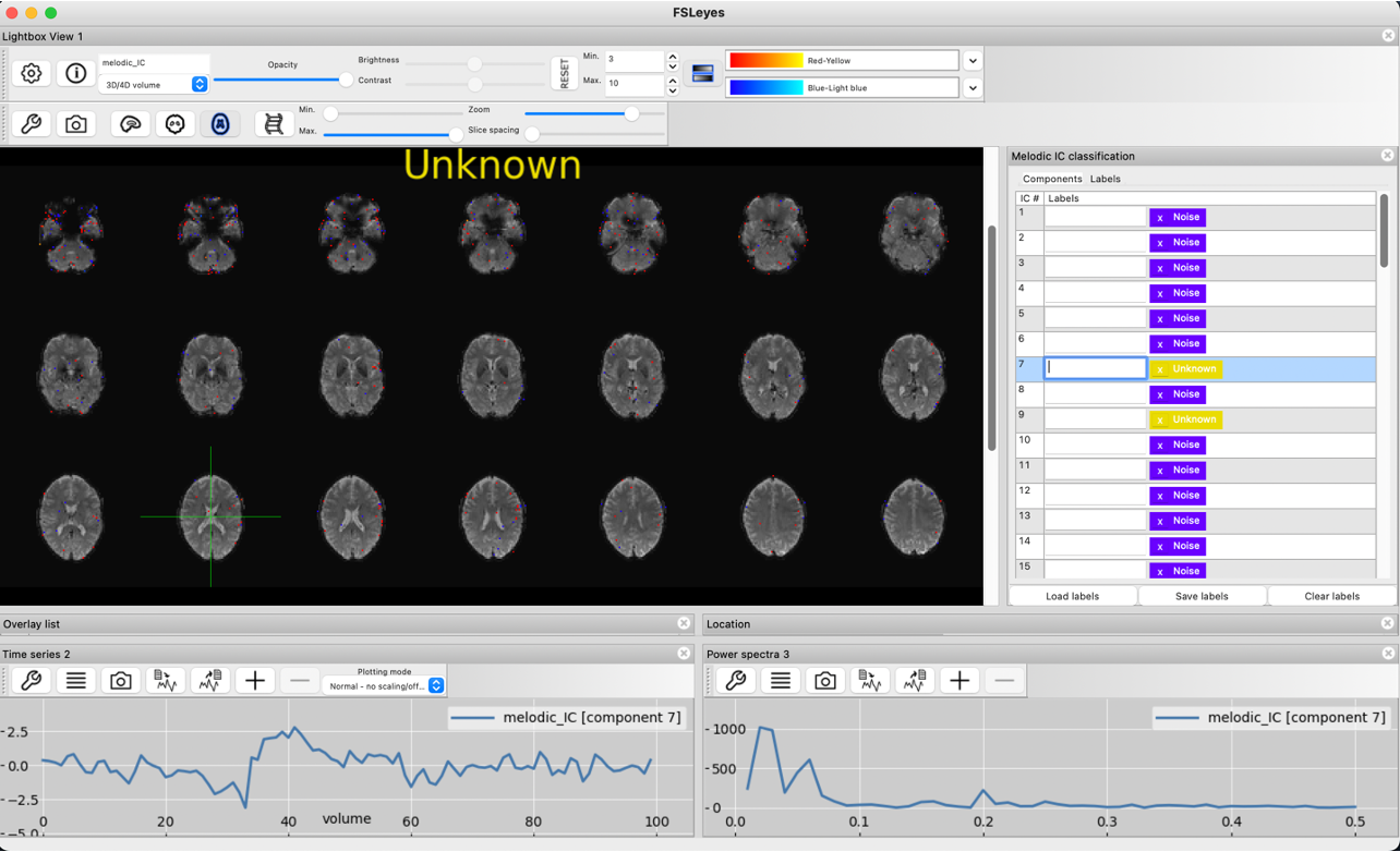
The below timecourse shows some signs of noise, but could also contain some signal. Because neither the spatial map, nor timeseries plot and power spectrum can definitively identify this component as noise or signal, this component is left unclassified.
Features to use for classification
Different spatial and temporal features can hint at components being noise-driven or signal-driven. The tables below give a summary of features that appear in the spatial map of the components. These features are also some of the features calculated by FIX for classifier training - in total FIX calculates ~180 features per component. I have covered using FIX to train a classifier for automated labelling and data cleaning in a separate blog post. Head over there to learn more about how to use your hand-labeled training set with FIX.
| Spatial feature | Signal characteristic | Noise characteristic |
|---|---|---|
| Clusters’ size and spatial distribution | Low number of large clusters | High number of small clusters |
| Voxels overlaying bright/dark raw data voxels | More overlap with GM intensity | Overlap with e.g. blood vessels |
| Overlap with brain boundary | Low overlap | High overlap |
| Overlap with different tissue types | Overlap with GM | Overlap with WM, CSF, vessels |
Features that appear in the time series plot and the power spectrum of the component are in the table below.
| Temporal feature | Signal characteristic | Noise characteristic |
|---|---|---|
| Jump (i.e. sudden changes) amplitudes in the time series | Fairly smooth time series | Large jump |
| Time series distribution | Fairly normal | Bimodal or long-tailed |
| Distribution of power in frequency domain (Fourier transform) | Low frequency | High frequency |
Saving classified component lists
When going through your components in the fsleyes melodic view, make sure to save your labels by clicking on the Save labels tab and giving it a name like hand_labels_noise.txt (required by FIX). If you want to train the FIX classifier with these labels, then the format with which fsleyes saves these files is ideal (info on the format requirements). You should label each component in each of the scans you are using to train FIX as either Signal or Noise or leave it as Unknown.
To loop quickly through a subset of scans for classification, I usually use this script:
data_dir=/path/to/your/data/resting_state/imaging_data/
design_dir=~/code/preprocessing/

subjects=(`ls -d ${data_dir}/s??`)

# ------ Classify single-subject ICA components ------
for i in $subjects; do
    subject=${i##*s}

    # test if subject is in ${design_dir}/classified_subjects.tsv
    if grep -q s${subject} ${design_dir}/classified_subjects.tsv; then
        run=`grep s${subject} ${design_dir}/classified_subjects.tsv | awk '{print $2}'`
        if [ -d $i/run${run}.feat/filtered_func_data.ica ] && [ ! -f $i/run${run}.feat/filtered_func_data.ica/hand_labels_noise.txt ]; then
                echo CLassifying $i ${run}

                # Open motion parameter plots either from report_prestats.html or generate them from rp_run_${run}.txt
                if [ -f  $i/rp_run_${run}.txt ] && [ ! -f $i/rot_${run}.png ]; then
                    fsl_tsplot -i $i/rp_run_${run}.txt -t 'SPM estimated rotations (radians)' -u 1 --start=1 --finish=3 -a x,y,z -w 800 -h 300 -o $i/rot_${run}.png
                    fsl_tsplot -i $i/rp_run_${run}.txt -t 'SPM estimated translations (mm)' -u 1 --start=4 --finish=6 -a x,y,z -w 800 -h 300 -o $i/trans_${run}.png
                    fsl_tsplot -i $i/rp_run_${run}.txt -t 'SPM estimated rotations and translations (mm)' -u 1 --start=1 --finish=6 -a "x(rot),y(rot),z(rot),x(trans),y(trans),z(trans)" -w 800 -h 300 -o $i/rot_trans_${run}.png
                fi
                if [ -f $i/rot_trans_${run}.png ]; then
                    open $i/*_${run}.png
                else
                    open $i/run${run}.feat/report_prestats.html
                fi

                fsleyes --scene melodic -ad $i/run${run}.feat/filtered_func_data.ica

            else
                echo "Already classified $i ${run}"
        fi
    else
        echo "Not classifying $i"
    fi
done
Links and Resouces
I picked up a lot that is covered here from excellent colleagues, including, but not limited to Ludo, Alberto, and the FSL Course Team. A special mention goes to Ludo’s fantastic teaching materials and papers on noise classification, which I have linked below:
Paper on Classifying Components: “ICA-based artefact removal and accelerated fMRI acquisition for improved resting state network imaging”
Educational course slides: “The Art and Pitfalls of fMRI Preprocessing”
FIX Classifier User Guide: Link
FEAT User Guide: Link