How to fieldmap correct
 Example Fieldmap in rad/s.
written for the Diedrichsen Lab & Brain and Mind Institute.
About this guide
Here I will describe the steps to create and apply fieldmaps to correct for epi distortions. I will focus particularly on the things you need to check in order to make sure you have done each step correctly, as there are a few pitfalls when doing the fieldmap correction.
For ideal results, I would recommend preparing the fieldmap and performing the combined unwarping and epi registration with the FSL FEAT tool. Once you have obtained the fieldmap and checked that the unwarping is correct, you can apply the fieldmap to any epi runs collected within the same scanning session (as long as the subject has not been taken out of the scanner between the fmap acquisition and the epi run). You are free to preprocess the epi run with the tools of your choosing (SPM, FSL, etc.) before applying the unwarping using your fieldmap.
This guide will work for fieldmaps acquired on a SIEMENS scanner. If you have another scanner type, then most of the steps are applicable, but the tool fsl_prepare_fieldmap for creating the fieldmap will not work. For help with non-SIEMENS data, have a look at this website.
Background
Briefly, air-tissue interfaces in the subject’s head (for example at the sinusses) cause magnetic disturbances, leading to a slightly inhomogenous B0 field. EPI acquisitions are quite sensitive to these deviations from a perfectly homogenous B0 field. A map of the B0 deviations is called a fieldmap. The fieldmap measures the B0 deviations and is acquired while the subject is in the scanner. It is later used to correct the EPI scan for the measurable B0 deviations.
B0 field inhomogeneities cause signal loss and signal distortion. We can only correct for signal distortion, not loss of signal. The direction of the distortion is the phase encode (PE) direction. We use the fieldmap to estimate the size of the distortion at each location along the PE direction and ‘put the signal back’ where it came from. We also use the fieldmap to estimate signal loss, to later make sure our registration ignores those areas where signal loss is too big.
For a detailed introduction into EPI distortion correction with fieldmaps, have a look at the FSL lecture slides and the FSL lecture. The FSL registration practical and the FSL distortion correction practical are also helpful.
Which images do I need to produce a fieldmap?
You will usually have two magnitude images and one phase image. To find out which is which, pull them up in your favourite image viewer and compare them to the images here:
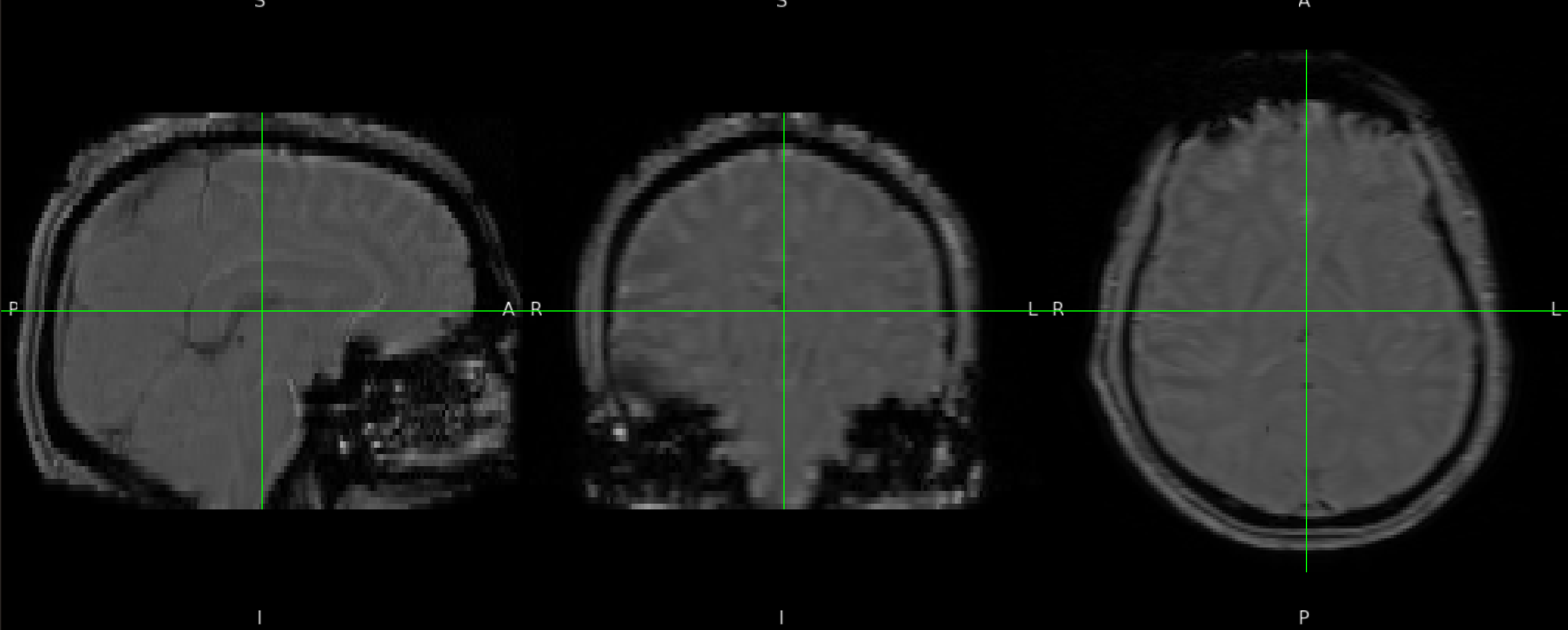 Example magnitude image.
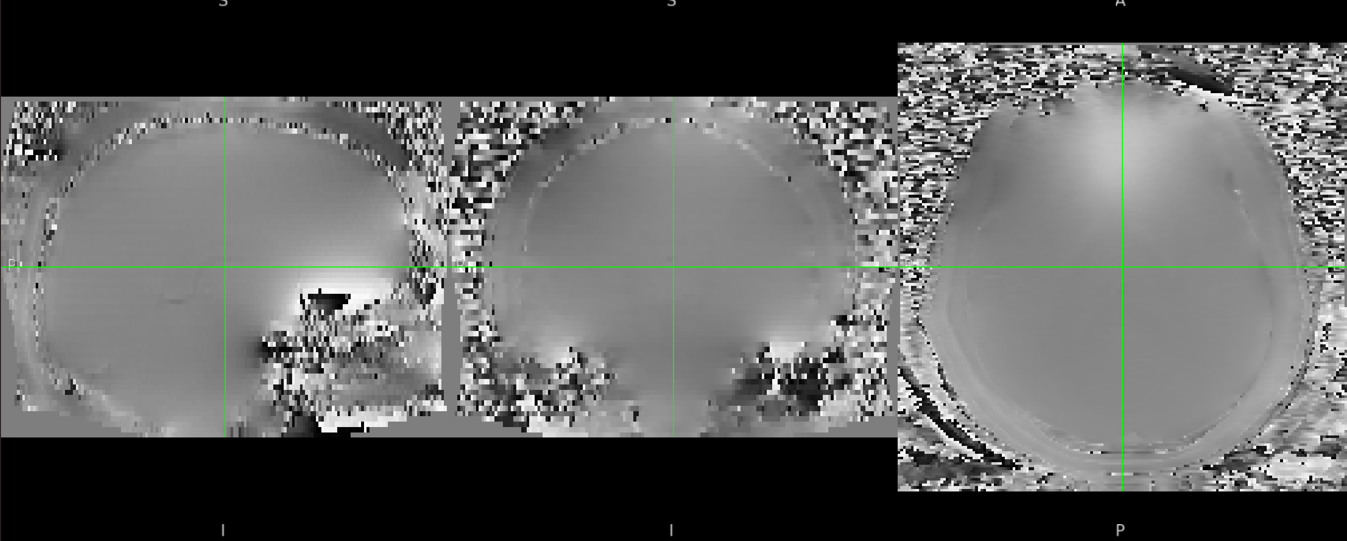 Example phase image.
Create fieldmap
To ease use of fsl tools, reorient the images to fsl-standard.
raw_dir=/path/to/your/input/directory
output_dir=/path/to/your/output/directory
subject=01
run=01

# Reorient fmap magnitude and phase image
if [ ! -f ${output_dir}/fmap/fmap_mag.nii.gz ]; then
  echo "Reorienting fmap"

  fslreorient2std \
  ${raw_dir}/fmap/sub-S${subj}_ses-1_run-01_magnitude2.nii.gz \
  ${output_dir}/fmap/fmap_mag

  fslreorient2std \
  ${raw_dir}/fmap/sub-S${subj}_ses-1_run-01_phasediff.nii.gz \
  ${output_dir}/fmap/fmap_phase

else echo "fmap already reoriented"
fi
Next, you need to skull-strip the fieldmap magnitude image. This is so that we can use the magnitude image as a mask to later exclude suprious voxels outside of the brain from the phase image.
Before we skull-strip the magnitude image, we want to make the magnitude image as homogenous as possible, to help the skull-stripping algorithm find the brain-nonbrain boundaries. We therefore run a bias correction on the magnitude image. Note that this bias correction is optional and you might not need it if regular skull stripping works fine on your magnitude image. So before going through the hassle of the bias correction, do an initial skull strip (code section under “Bet fmap magnitude image”) and see if you’re happy with the result. If not, fsl_anat has a good bias correction implemented (as part of FAST). Since we’re not interested in anything but the bias correction, we’re turning of cropping, segmentation and registration to standard (normalization).
This will take a few minutes to run, so submit the command and go for a coffee break.
# Run bias correction on fmap magnitude image
if [ ! -d ${output_dir}/anat/fmap.anat ]; then
  fsl_anat \
  --strongbias  --nocrop  --noreg  --nosubcortseg  --noseg \
  -i ${output_dir}/fmap/fmap_mag \
  -o ${output_dir}/fmap/fmap;
  echo "Running fsl_anat on fmap"
else echo "fsl_anat on fmap already run";
fi
fsl_anat has created a folder fmap.anat, in which you can find the bias-corrected magnitude image. The image is called T1_biascorr.nii.gz. Ignore the naming of the file, this is because fsl_anat assumes that you have passed it a T1 image.
Now we’re ready to skull-strip. I use the fsl tool BET (brain extration tool) with the “-R” flag to get a recursive skull-stripping.
# Bet fmap magnitude image
bet \
${output_dir}/fmap/fmap.anat/T1_biascorr \
${output_dir}/fmap/fmap_mag_brain_bet -R
BET is slightly more lenient than we would like it to be in this case. Usually, we want to make sure we definitely include all brain voxels into the skull-stripped image. But for the fieldmap, we want to be very conservative and exclude any non-brain voxels from the image. That is because the we don’t want spurious voxels in the phase image that lie outside of the brain to affect our fieldmap. And the fieldmap is going to be extrapolated, so even if we exclude brain voxels, they will be included into the fieldmap.
Therefore, we are going to erode the skull-stripped magnitude image and choose the skull-stripped version that excludes all non-brain voxels.
fslmaths \
${output_dir}/fmap/fmap_mag_brain_bet -ero \
${output_dir}/fmap/fmap_mag_brain_ero1

fslmaths \
${output_dir}/fmap/fmap_mag_brain_ero1 -ero \
${output_dir}/fmap/fmap_mag_brain_ero2
Now pull up the skull-stripped magnitude image, and your two eroded versions over the phase image in your image viewer to choose the best skull-stripped version. I start by looking at the most lenient version that includes the most voxels and see whether it covers any spurious voxels of the phase image. If it does, I go to the next more conservative version and check the same. I usually settle on the skull-stripped magnitude image with 1 voxel eroded (fmap_mag_brain_ero1.).
Once you have chosen your best skull-stripped image, set this as the variable chosen_brain_extraction.
fsleyes  \
${output_dir}/fmap/fmap_phase \
${output_dir}/fmap/fmap_mag_brain_bet \
-dr 0 1 -a 50 -cm blue-lightblue \
${output_dir}/fmap/fmap_mag_brain_ero1 \
${output_dir}/fmap/fmap_mag_brain_ero2 \
-dr 0 1 -a 50 -cm red-yellow &

chosen_brain_extraction=${output_dir}/fmap/fmap_mag_brain_ero1
To abide by the naming convention that FSL’s FEAT needs, we rename the chosen skull-stripped magnitude image fmap_mag_brain.nii.gz. Your non-stripped magnitude image needs to be named fmap_mag.nii.gz (the .nii.gz suffix is missing in the code because FSL tools automatically assume that images have that ending. If yours end in .nii, then try running gzip ${output_dir}/fmap/fmap_mag before applying the FSL commands.
# Copy the skull-stripped and non-stripped magnitude image and rename them
fslmaths ${chosen_brain_extraction} ${output_dir}/fmap/fmap_mag_brain
fslmaths ${output_dir}/fmap/fmap.anat/T1_biascorr ${output_dir}/fmap/fmap_mag
(You don’t have to use fslmaths for this operation, since we are not doing anything to the image other than copying and renaming it. You can use cp for this operation or simply copy and rename in whatever file manager you use. I just got into the habit of using fslmaths, since you won’t need to specify the file ending.)
The last parameter you need for preparing the field map is the echo time difference of the fieldmap sequence. You will pass this to the fsl_prepare_fieldmap command. This depends on your fieldmap acquisition. You should be able to find the two echo times for the field map acquisition in the scanning protocol (see screenshot below). Simply subtract the smaller from the bigger echo time to get the echo time difference. Otherwise you can find out this parameter from your scanner operator (defaults are usually 2.46ms on SIEMENS, but not always).
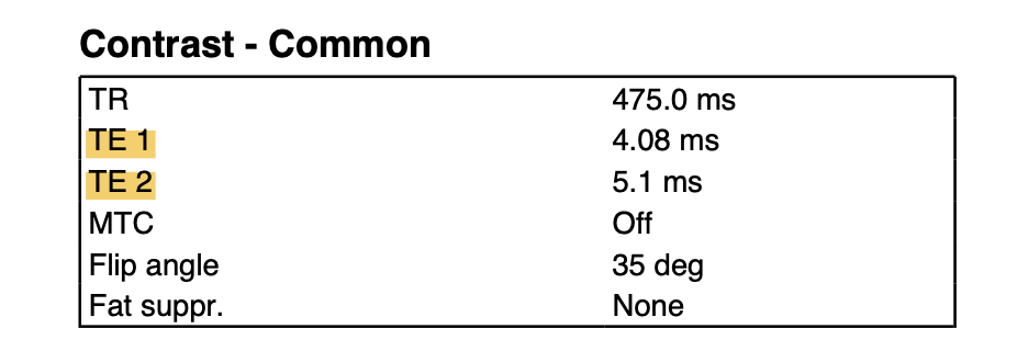 Scanning protocol section with field map parameters.
Now we will pass the phase image, magnitude image, and skull-stripped magnitude image to fsl_prepare_fieldmap to create a fieldmap suitable for FEAT saved in rad/s.
# Generate fieldmap
fsl_prepare_fieldmap SIEMENS \
${output_dir}/fmap/fmap_phase \
${output_dir}/fmap/fmap_mag_brain \
${output_dir}/fmap/fmap_rads 1.02
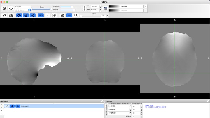
Inspect your fieldmap (fsleyes ${output_dir}/fmap/fmap_rads &) and make sure it looks ok. It should look something like the fieldmap shown in the second figure of the FSL distortion correction practical.
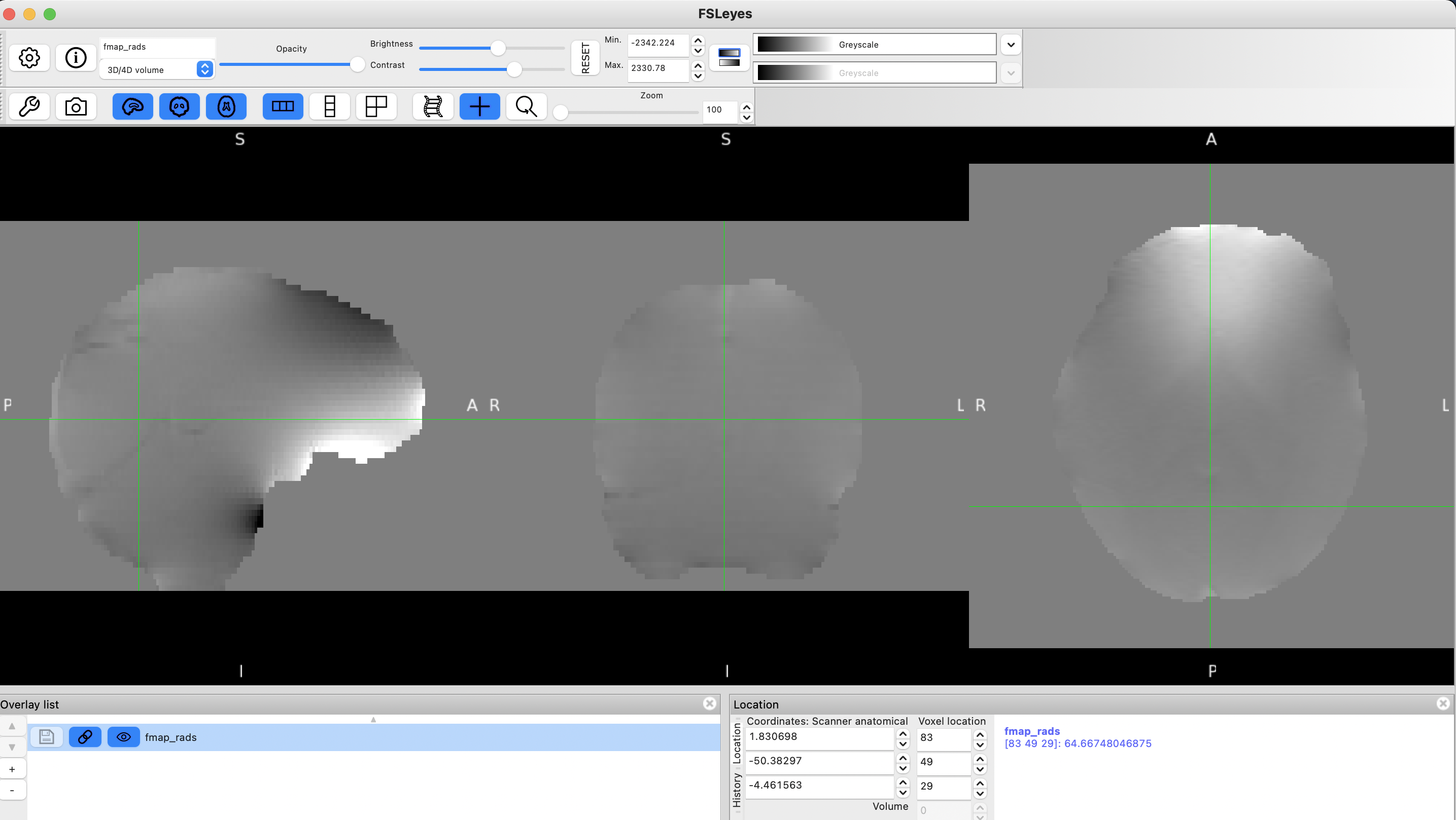 Example fieldmap in rad/s.
Apply fieldmap
Once you have created your fieldmap, you can use it to correct your epi data with FSL’s FEAT.
If you do this for the first time, pull up the FSL FEAT GUI and the User Guide, then set the analysis to ‘First-level analysis’ and ‘Preprocessing’. I would recommend going through each required field and reading the ‘balloon help’ window that pops up when you hover over the field. Select the right scans and fill in your scan parameters for each window.
For the fieldmap correction, select ‘B0 unwarping’. In the fields that pop up, select your fieldmap in rad/s you created earlier (in our example it’s called fmap_rads.nii.gz) and the skull-stripped magnitude image. It should be in the same folder as your non-skull-stripped magnitude image and end in ‘_brain.nii.gz’.
Fill in the effective echo spacing (also known as ‘dwell time’) and the echo time. The balloon help field will tell you more about both parameters. To find these out for your sequence, a good starting point is having a look in the scanning protocol (you can get that from your scannner operator). This article will also help you understand and locate the parameters. Note that if you have an accelerated sequence, the effective echo spacing is the echo spacing divided by the acceleration factor. To find out if you have an accelerated sequence (e.g. GRAPPA acceleration), refer to your scanning protocol or ask your scanner operator.
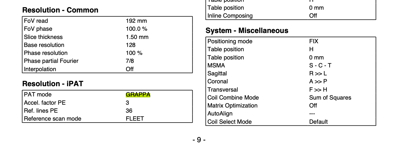 Example page of a scanning protocol. GRAPPA parameters are found in the bottom left corner.
If you work with data that comes with an associated json file, you will likely be able to find the effective echo spacing in the json file:
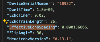 Example json file.
If the fieldmap correction has gone wrong (too much or too little correction), the effective echo spacing is one of the first parameters to check.
One parameter which you will likely have to try out is the unwarping direction. The PE direction for the example data was the z dimension. But it is not immediately obvious whether you have to unwarp in the plus or minus z direction. Therefore, run the FEAT separately for both directions and then compare the results. You can tell from visual inspection whether the unwarping has made the distortions better or worse. Visual inspection of the distortion correction is described below.
After you have filled in all of your parameters and data paths for the preprocessing, save the preprocessing design file (click Save in the GUI). This will give you a .fsf file that you can load into the FEAT GUI again to process this or other runs. With the .fsf file, you can also run the preprocessing from the command line, by running feat design.fsf. The design file will also help script your analysis once you have established a working pipeline.
To script your analysis for several subjects, sessions and runs, open the design.fsf file with a text editor. Replace all the subject IDs with XX, all the session IDs with YY and all the run IDs with ZZ and save the design.fsf as a template file (e.g. fmap_design.fsf). For an example template file, look at this file.
Then, after creating your fieldmap and all other necessary images for the preprocessing, you can create a subject-session-and-run-specific design file and fill in all the identifiers:
# ---- Create design file for preprocessing func run ----
designs=${workdir}/Cerebellum/Pontine7T/code/pontine_7t/designs
session=$(echo ${ses} | sed 's/^0*//')

# Make copy of template design file
cp ${designs}/fmap_design.fsf \
${designs}/fmap_sub-${subj}_ses-${ses}_run-${run}.fsf

# Fill in subject-session-and-run-specific parameters
sed -i " "  \
"s/XX/${subj}/g" "${designs}/fmap_sub-${subj}_ses-${ses}_run-${run}.fsf"

sed -i " "  \
"s/YY/${ses}/g" "${designs}/fmap_sub-${subj}_ses-${ses}_run-${run}.fsf"

sed -i " "  \
"s/ZZ/${run}/g" "${designs}/fmap_sub-${subj}_ses-${ses}_run-${run}.fsf"
Then you can run the preprocessing:
feat \
"${designs}/fmap_sub-${subj}_ses-${ses}_run-${run}.fsf"
You need to make sure that the paths in your design file are appropriate for the server you want to run your analysis from. That means, if you create your design file locally, with the data server that contains your data mounted and then try to run the analysis from the robarts server, the analysis will fail. That’s because locally, your paths begin with something like ‘/Volumes/diedrichsen_data$/data/…’, but on the robarts server your paths begin with ‘/srv/diedrichsen/data/…/
You can check that your design file has the correct paths by pulling up the FEAT GUI on the robarts server (or wherever you want to run your analysis from), then loading the subject-session-and-scan-specific design.fsf file and clicking ‘Go’. FEAT will show you an error message if your paths are not correct. If your analysis is set up correctly, a webbrowser window will open and your analysis will start running.
I would advise you to first make sure the fieldmap correction has worked correctly on an example subject (using the steps below) and then moving on to scripting the analysis for all subjects, sessions and runs.
Check fieldmap correction
The output from the preprocessing is found in the output folder you set (GUI field ‘Output directory’) with the suffix ‘.feat’. For example, for my example design.fsf file, the output is located in /srv/diedrichsen/data/Cerebellum/Pontine7T/derivatives/sub-02/ses-1/func/run-01.feat. The distortion-corrected data is filtered_func_data.nii.gz
We want to make sure that the fieldmap correction has worked correctly, so we are going to pull up the report.html. Point your browser at the file (open /srv/diedrichsen/data/Cerebellum/Pontine7T/derivatives/sub-02/ses-1/func/run-01.feat/report.html) or open the folder and double-click report.html. In the webbrowser, click on ‘Registration’ and then ‘Unwarping’.
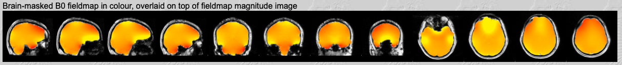 Fieldmap in colour.
The first row shows a colour map of the fieldmap. This should be fairly uniform, except in the inferior temporal and frontal areas.
Fieldmap in colour.
The first row shows a colour map of the fieldmap. This should be fairly uniform, except in the inferior temporal and frontal areas.
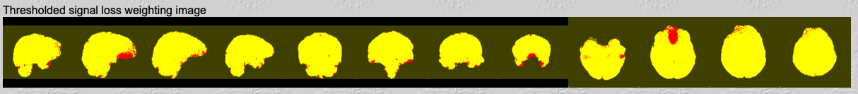 Signal loss map.
In the second row you’ll see a map of the areas that are ignored for the registration because of their signal loss. We expect to see red in those inferior temporal and frontal areas, where there is the most signal loss. We don’t expect to see too much of it, because if too much of the brain is being ignored for registration, then our registration won’t look good. But if you have no signal loss here, that also usually means something has gone wrong in your pipeline, since we expect to see a little bit of signal loss.
The example data used here was acquired with a OP coil (occipital-parietal coil). This coil is focussed on the back of the brain (posterior areas). Therefore the signal loss at the frontal areas is particularly bad and those are ignored more than usual. If you have a wholehead coil, signal loss in the frontal areas should not look this bad.
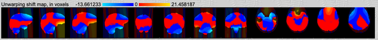 Voxel shift map.
In the third row you can see by how much the voxels are shifted. First, look at the range of voxel shift. This should be between +/- 3 to +/- 20. If the shift has an exorbitant high range, then something went wrong. Check the calculation of your effective echo time (did you remember to divide by the PE direction acceleration factor?) and check that the fieldmap you created is in radians per seconds (rad/s). Usually, if the voxel shift range is really high, then something went wrong with the units of the fieldmap or the parameters you are putting in for the echo time spacing. However, the range indicates the maximum voxel shifts. Looking at the example shift map, you can see that only very few voxels in the frontal areas were shifted by this maximum amount. All other voxels were shifted by only a few (perhaps 1-5) voxels.
In the shift map you can also see the direction of the unwarping. A negative voxel value means that signal from this voxel was pulled in the decreasing PE direction, so the direction where the voxel coordinates decrease. For example, in our example data the PE direction is the z-direction and the z coordinates decrease in the inferior direction. A negative value for a cerebellar voxel in our data indicates that signal from this voxel was pulled more inferior. Conversely, a positive voxel value from the occipital lobe indicates that signal from this voxel was shifted superiorly.
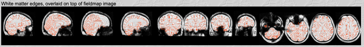
You can see the effect of the unwarping even better when scrolling all the way down to the unwarping gif.
This gif is flipping between the unwarped epi image and the distorted epi image (marked by a red dot). Both images were registered to the structural image, and have the white matter edges of the structural images overlaid on top of the epi image. Look at the shift between the unwarped and the distorted epi image - does the unwarping make the image look ‘more brain-like’ or does it make the distortions worse? You should be able tell whether the direction of the distortion was correct from comparing a distortion correction in the minus PE direction to a distortion correction in the plus PE direction.
For closer inspection, pull up these images in fsleyes. Pick an area that experiences a large voxel shift (but not one that has been ignored due to too much signal loss!). Then flip between the images and the structural image to see whether the distortion correction brings the epi image closer to the ‘ground truth’, i.e. the structural image. Below, I describe how to do this for cerebellar areas.
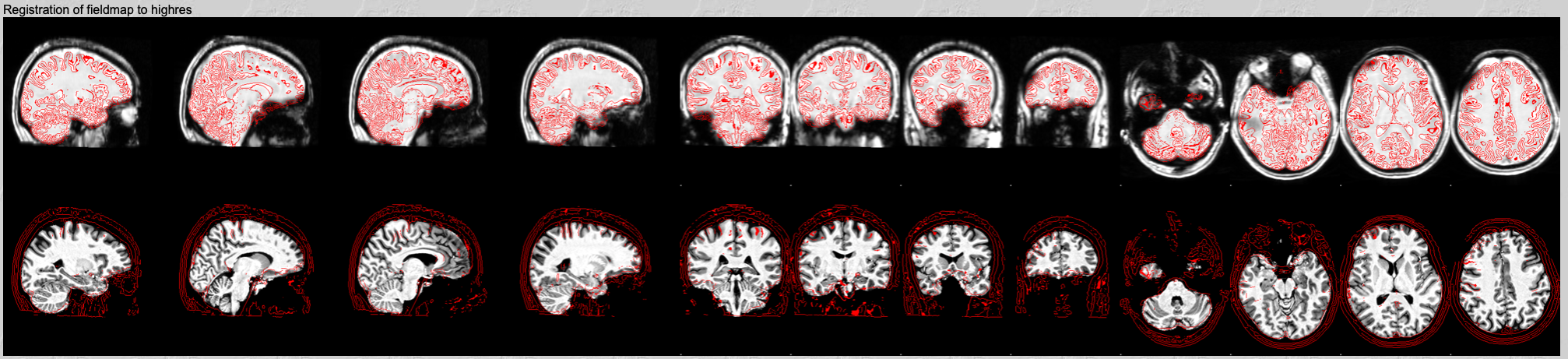 Fieldmap magnitude to structural registration.
In the fourth row you can check the registration of the fieldmap image to the structural. It shows the fieldmap magnitude image registered to the structural, with the white matter edges from the structural overlaid on top. This should usually have worked well and you just need to do a quick check that everything looks right. If not, check your inputs: Have you named the skull-stripped fieldmap image and non-skull-stripped fieldmap image correctly? Does your structural image looks good (bias-corrected, nicely skull-stripped, named correctly)?
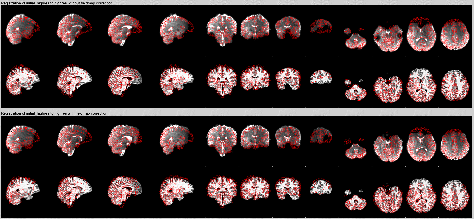 Registration of initial_highres to highres with and without fieldmap correction.
Finally, this is where you can directly compare the registration results with and without the fieldmap correction. The white matter edges (red lines) should align better with the GM-WM boundaries on the greyscale image after applying the distortion correction.
For a more detailed comparison in fsleyes, follow the instructions at the bottom.
Note that if you have not used an sbref image (see above), then these images are titled ‘example_func to highres’.
CHECKING CEREBELLAR SIGNAL
The cerebellum is especially vulnerable to distortions due to B0 Field inhomogeneities, because it is located close to the air-tissue interfaces that cause magnetic disturbances. To check that the unwarping did a good job for the cerebellum, pull up the structural image, the fieldmap-corrected epi image and the uncorrected epi image (both registered to the structural):
cd ${output_dir}

fsleyes \
func/run-01.feat/reg/highres.nii.gz \
func/run-01.feat/reg/unwarp/initial_highres_distorted2highres.nii.gz \
func/run-01.feat/reg/initial_highres2highres.nii.gz &
(In my data, I am using the sbref image - called ‘initial_highres’ by FSL - to get a better registration of the epi data to the structural. If you don’t have an sbref image that is different from your epi images, then you want to pull up example_func_distorted2highres.nii.gz and example_func2highres.nii.gz instead.)
Then adjust brighness and intensity of the epi images so that you can see where most of the epi signal comes from. Put your cursor at the most inferior point from which the cerebellar epi signal is coming from in the uncorrected epi image and toggle between that image and the structural. Does the epi signal end where the cerebellar structure ends? Now have a look at the corrected epi image and place your cursor at the most inferior point of the lateral cerebellar epi signal. Toggle between this image and the structural. Does the epi signal end closer to where the cerebellar tissue ends in the structural? If so, then the fieldmap correction helped put the signal back where it came from. We will never be able to recover the epi signal from these inferior cerebellar areas fully, as there is signal loss in these areas. But we should be able to correct the signal distortions in those scans if the fieldmap was applied correctly.
Acknowledgments
A lot of the content covered here I’ve learned during my time participating in and later teaching on the FMRIB FSL Course. I highly recommend checking out their lectures, practicals and tutorials - and attending in the course if you find yourself in Oxford!