How to clean fMRI data with FIX-ICA

About this guide

This post guides you through ICA-based cleaning of fMRI data. I focus here on the practical steps, quality inspection and troubleshooting tips rather than the theoretical background. For a deeper dive into the methods and the tools used here, check out the resources linked at the end. For ICA component classification, have a look at this post.

• Background
• Running the single-subject ICA
  • Creating the template design file
  • Generating scan-specific design files
  • Running the scan-specific design files
  • Checking registrations
• Classifying components
  • How many scans do we need to classify?
• Training FIX
• Leave-one-out Testing
• Applying FIX
• Addendum: Checking how FIX affected cerebellar correlations
• Links and Resouces

Background

In resting-state fMRI processing, we often apply Independent Component Analysis (ICA) to clean the data from noise. All fMRI data suffers from unwanted noise, but resting-state fMRI has the additional challenge of lacking any kind of information about when relevant signals should occur. This is in contrast to task-based fMRI, where the task regressors tell us when to expect fluctuations in the BOLD signal that are related to neural processes. Therefore, resting-state fMRI is much more reliant on removing noise from different sources such as head motion or body functions. Various methods exist, such as using external recordings of bodily functions (for example physiological recordings of heart rate and breathing). But in the absence of any external recordings, data-driven methods such as ICA offers a useful method that separates true brain signals from structured noise.

ICA is a dimensionality reduction method, similar to Principal Component Analysis (PCA). That means, ICA reduces the high-dimensional raw functional data into a low-dimensional representation. Put differently, ICA finds patterns in the data that are independent form each other and explain substantial variance in the data. By breaking down the data into these patterns, or components, ICA separates the data into components that reflect BOLD signal and components that reflect noise (physiological, imaging reconstruction artefacts, movement, etc.).

ICA components consist of a single 3D spatial maps and an associated time course. Using the map, the timecourse and a frequency domain representation of the timecourse, we can identify the noise components, label them, and regress their associated variance out of the raw data - thereby removing the noise.

A single 10-minute resting-state scan of good quality (TR of 1 and 2.5mm isotropic voxels) yields about 100-150 components. Wiith 20 subjects, we would need to manually label 2000 - 3000 components, which is very time-consuming. FMRIB’s ICA-based Xnoiseifier (FIX) offers an automated ICA-based cleaning approach. It is a classifier that can automatically label components as noise or signal. For studies that use HCP-data or data that is matched to HCP data in study population, imaging sequence and processing steps, it works out of the box. But for most applications that deviate from the HCP or other commonly used protocols slightly, FIX has to be trained on hand-labelled data. Check out the FIX User Guide to see if you can use an existing training dataset and the FAQ to see which one. This post will walk you through generating your own training dataset for FIX by hand-labelling a set of scans from your own data, training FIX on it and applying FIX to your functional data for noise removal. If you are able to use an existing FIX dataset, you will still need to go through most steps in this procedure, but you can leave out the noise classification and training of FIX.

We can also apply ICA-based cleaning to task fMRI. However, because of the effort involved this is usually not done for standard task-based fMRI studies and only applied to resting-state fMRI where we really need the signal strength. But nothing is stopping you from trying it out on task!

Running the single-subject ICA

In this post, I will be working with resting-state fMRI data from 19 subjects, each of which had 2 runs of 10 minutes acquired. To run the single-subject ICA, I will run the ICA on each of the runs of each subject separately. Each run gets processed separately, since some structured noise components might differ between runs. And of course, they will differ between subjects.

Creating the template design file

If you have a lot of data to run through the single-subject ICA steps, then it is advisable to create a template ICA file and generate the scan-specific version by filling in the necessary details using a script. I will walk you through these steps here.

Start by creating a design file for a single subject. Run Feat_gui & from the command line (or Feat depending on which machine you’re using). Set the analysis to First-level analysis and Preprocessing. Select the functional scan in the Select 4D data tab. Check that the TR is correct. The TR is being automatically read out form the header. If incorrect, you need to correct the header (use fsledithd or nibabel for this). Also check that the total volumes match. Set the volumes to delete to the number of dummy scans to remove from your images. If you don’t know if you have already removed the dummy scans from your acquired images, check whether the intensity changes dramatically between your first image and your 20th, 50th or 100th image in fsleyes. If there is no large change, you can keep all images - though it’s also fine to remove the first 10 or so images if you wish to be on the safe side. This is how the Data tab looks like for my data:

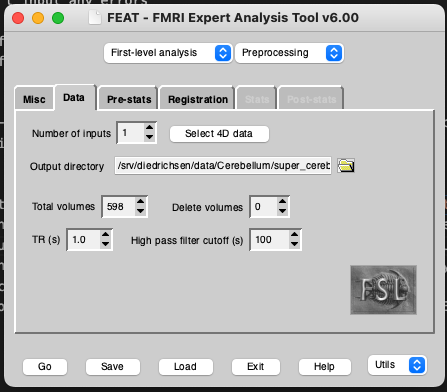
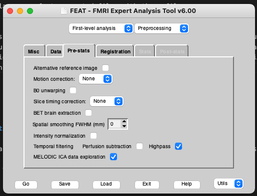
Make sure that you turn off all preprocessing steps that are turned on by default in the FEAT GUI that you have already run or that you don’t want for your data. For example, if you are using functional data that has already been motion corrected, set Motion correction to ‘None’. Also be sure to turn of spatial smoothing by setting Spatial smoothing FWHM (mm) to 0. To run single-subject ICA turn on MELODIC ICA data exploration.

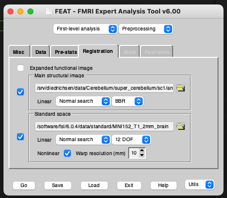
To ensure that FIX can train on your classified data, you need to run registrations from func space to standard space, ideally via a high resolution T1 (so func2highres and highres2standard to get func2standard). You can either run your own registrations with the non-FSL program of your choice and make them FSL-compatible (I will provide a blog post on this in the future) or you can run the registrations within FEAT by turning it on in the Registration tab. These registrations don’t need to be perfect if you are only going to be using them for FIX classification, since FIX just needs an approximately accurate mapping from functional to standard space to pull 3 standard-space masks of the major veins into functional space (check out the FIX paper for details). These masks are later used for feature extraction for the FIX classifier. If you choose to go with FEAT-generated registrations (which is usually the most convenient option), I would recommend using BBR registration from the functional to the highres image. FEAT needs a brain-extracted highres image for this along with the whole-head image. For best results, use optiBET to get the most accurate extracted image, then rename this to end in _brain.nii.gz and input it as your highres image for FEAT. Importantly, FEAT needs to be able to find your whole-head image in the same folder with the same name, but without the _brain suffix (So if your highres is called highres.nii.gz, it needs to be in the same folder as your brain-extracted highres_brain.nii.gz image).

To make sure that you have set all files to valid filenames, save your design file and wait to see if any error messages are coming up. If you are setting up your filenames to run on a different machine or server, but you are not currently on that server then of course you will get some error messages but it should still run through. In that case, try to do this final check from the machine on which you will be running the FEAT program from.

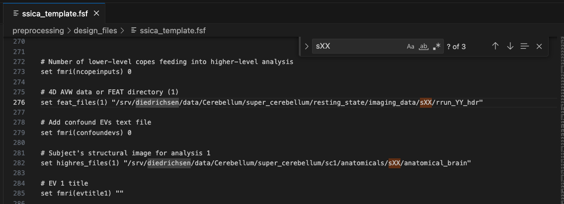
Once everything is correct, save this file as ssica_template.fsf. Open the file in your favourite text editor and replace all scan-specific information by variable names that are used NOWHERE ELSE in the file. You don’t want to accidentally change something other than your scan-specific information. I usually set every subject identifier to ‘XX’, every session identifier to ‘YY’ and every run identifier to ‘ZZ’. Since there are no session identifiers in the case of my data, I use ‘XX’ for subject and ‘YY’ for run, as you can see here:

Generating scan-specific design files

After you’ve generated your design template, it’s time to loop over your subject identifiers and run identifiers (+ session identifiers if you have them) and fill the variables with these values. You can do this in bash using sed:

data_dir=/path/to/your/data/
design_dir=/path/to/your/design/file/

for i in ${data_dir}/s*; do
    for run in $runs; do
        subject=${i#*imaging_data//s}           
            cp ${design_dir}/ssica_template.fsf ${design_dir}/rest_${subject}_run-${run}.fsf
            # Fill in subject-and-run-specific parameters
            sed -i  "s/XX/${subject}/g" "${design_dir}/rest_${subject}_run-${run}.fsf"
            sed -i  "s/YY/${run}/g" "${design_dir}/rest_${subject}_run-${run}.fsf"
    done
done

Or you can do it in Python:

rest_dir = Path(f'/path/to/your/data/')
design_dir = Path(f'/path/to/your/design/file')

def make_design(subject, run):
    """Create the design file for the single-subject ICA for the subject and run.

    Args:
        subject (string): subject ID
        run (string): run ID
    """

    img_file = Path(f"{rest_dir}/s{subject}/rrun_{run}_hdr.nii.gz")
    design_template = Path(f"{design_dir}/ssica_template.fsf")
    design_output = Path(f"{design_dir}/ssica_{subject}_run-{run}.fsf")

    if img_file.is_file() and not design_output.is_file():
        # Read the contents of the template file
        with open(design_template, 'r') as template_file:
            design = template_file.read()

        # Replace placeholders in fsf content
        design = design.replace('XX', str(subject))
        design = design.replace('YY', str(run))

        # Write the modified content to the output file
        with open(design_output, 'w') as output_file:
            output_file.write(design)

for subject_path in rest_dir.glob('s[0-9][0-9]'):
    subject = subject_path.name[1:]
    for run in runs:
        make_design(subject, run)

Running the scan-specific design files

Once you’ve created all of your scan-specific files, do a few spot checks to make sure that everything is in order by calling the FEAT GUI, loading a scan-specific design file and saving it again. If no error messages pop up, you’re good to go!

To run the design files, you can again loop through your subject and run parameters and call the design file at each iteration:

data_dir=/path/to/your/data/
design_dir=/path/to/your/design/file/

for i in ${data_dir}/s*; do
    for run in $runs; do
        subject=${i#*imaging_data//s}
            echo "Running SS melodic for subjec ${subject} ${run}"
            feat "${design_dir}/rest_${subject}_run-${run}.fsf"
    done
done

To do this in Python instead, use a system’s call subprocess.Popen(['feat', str(design_output)]). We use subprocess.Popen() instead of subprocess.run(), since we don’t want to wait for the command to finish - Feat is going to take a while until it has finished the registrations and completed the single-subject ICA.

You can of course also load each design file into the FEAT GUI and just click on Go, but this is going to take a while and you could overlook one. However, if the command line is giving you trouble or if you simply want to re-run a single design file, doing it through the GUI is going to be a hassle-free option.

Checking registrations

Your single-subject ICAs have finished and you will want to dive into classifying the components. But hold your horses - first have a look at the reports. Open the report_log.html created under the output.feat folder (you specified a name for this folder in your design file). Have a look at whether any fatal errors have occurred during the processing. If so, the header of the page will say Error occurred during the analysis. If a non-fatal error occurred, then the Log tab of your report will show you the error and the command that produced it. However, most of the following steps were still able to run normally. In both cases, try to get to the bottom of the issue and re-run the design file with it fixed.

Even if FEAT ran smoothly, don’t move on just yet. Go to the Registration tab and look at the quality check images. Do your registrations from func2standard look good? If not, is the problem at the func2highres stage or the func2standard stage? Could it be a result of a previous preprocessing stage?

Here, we can see in the first image of the report that the registration from functional to standard space went wrong:

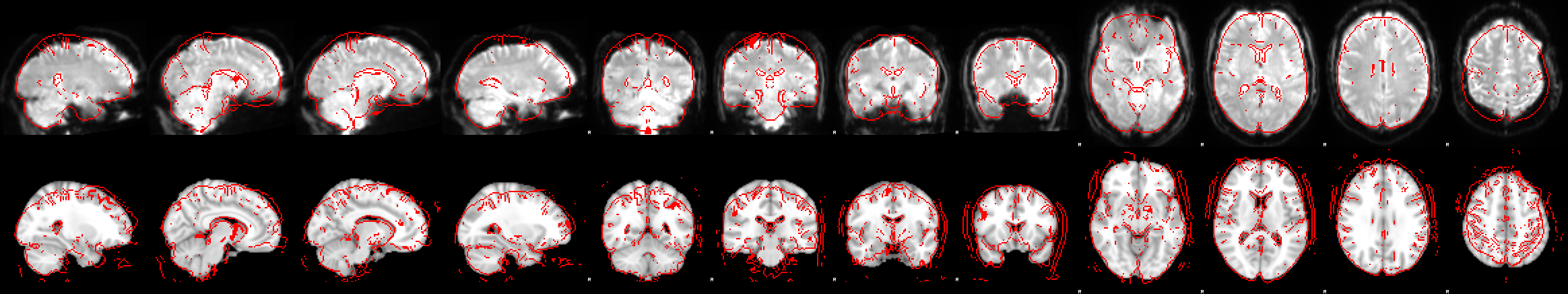
The next image which shows the example_func2highres stage, tells us what went wrong:

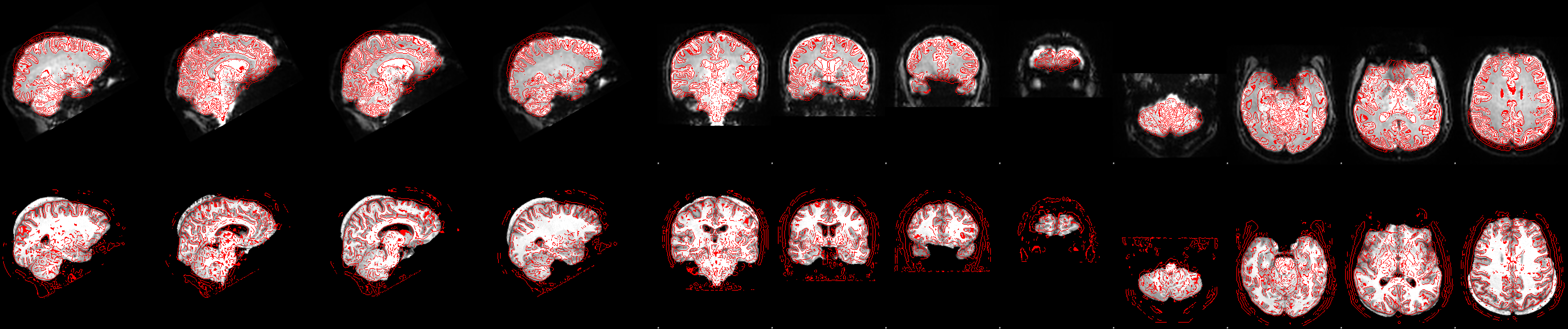
In the bottom row of the image above we can see the functional image (red outline) registered onto the highres image (greyscale image). The brain extraction of the highres image left a big chunk of skull at the back of the head. While the functional to highres registration is largely unaffected by this (we can see that the red outlines still match the underlying highres image pretty well) this left-over non-brain tissue messes up the registration of highres image to standard space:

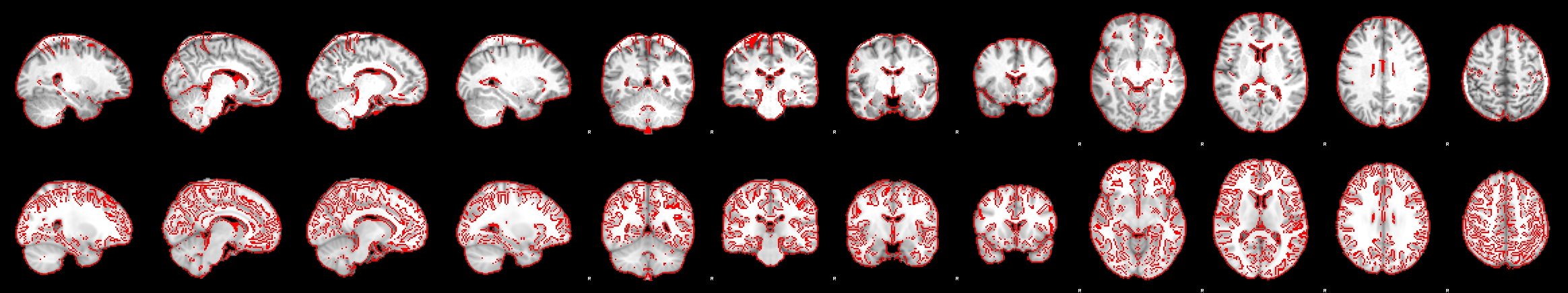As you can see, the nonlinear registration has squeezed the brain-extracted highres image so that it fits into the standard brain. To fix this, go back to the brain extraction, correct it so that the non-brain tissue is removed (optiBET, BET with different parameters or even hand correcting the brain mask can help) and re-run the registrations. Only the registrations need to be re-run, since the ICA is unaffected by messy registrations. So to save time, you can turn off the MELODIC ICA data exploration in your design file that you’re going to re-run now for this subject. After re-running, replace the reg folder in your original output.feat folder that holds the single-subject ICA for this subject with the reg folder from the re-run output folder.

Other issues that might pop up are faulty registrations because of wrong orientations of the image (try increasing the search to Full search), partial FOV of the functional images (try decreasing the DOF to 3 DOF), or suboptimal registrations because of anatomical abnormalities (consider constructing a study-specific template as a group template to register to). Most of these cases are covered in the FEAT User Guide, so head there for troubleshooting tips.

If you used fieldmaps in your registration, there are a few more plots to check at this stage. Head over to the post on fieldmap correction near the end of the page to find out which plots to inspect and what to pay attention to.

Classifying components

Now it’s time to classify the components of a subset of the scans into noise and signal. To ensure that we are not biasing our training set towards a particular group of subjects, sessions, timepoints or runs, we first need to generate a balanced subset of scans to classify. That is, our training set should consist of equal number of patient and control scans (if we have a patient and control group), pre and post timepoints (if we have two or more timepoints) and first and second runs (if we have more than one run). I like to create a .tsv file that contains the scans I have selected for classification.

def balanced_subset(subjects, runs, percent_data):
    # Calculate the number of subjects to select
    num_scans = len(subjects) * len(runs)
    num_scans_to_select = int(num_scans * percent_data * 0.01)

    # Generate all combinations of subjects and runs
    all_combinations = list(product(subjects, runs))

    # Shuffle the combinations to ensure randomness
    random.shuffle(all_combinations)

    # Initialize counters
    selected_subjects = set()
    subset = []

    # Select subjects while maintaining balance across runs
    for subject, run in all_combinations:
        if subject not in selected_subjects:
            selected_subjects.add(subject)
            subset.append((subject, run))

        if len(selected_subjects) == num_scans_to_select:
            break

    # Separate the subset into lists of subjects and runs
    subset_subjects, subset_runs = zip(*subset)

    return list(subset_subjects), list(subset_runs)
    
subject_list = [subject.name for subject in rest_dir.glob('s[0-9][0-9]')]
percent_data = 30
subset_subjects, subset_runs = balanced_subset(
    subject_list, runs, percent_data)
# Save
df = pd.DataFrame({'subject': subset_subjects, 'run': subset_runs})
df = df.sort_values(by=['subject', 'run'])
df.to_csv(f"{design_dir}/classified_subjects.tsv", index=False, sep='\t')

How many scans do we need to classify?

The more scans you classify, the better, but a general recommendation is to classify scans from at least 10 subjects. I usually aim for a subset of the data of 20-40%, depending on how many scans I have and how heterogenuous my sample is. For example, in the case of low quality patient data I would err on the side of classifying a larger subset of the data than when I have a dataset of high quality healthy control scans. But it’s also possible to train the FIX classifier, evaluate its performance, and then classify a few more scans if FIX does not perform well.

For a detailed explanation of how to classify ICA component, have a look at this post. There is also a fantastic paper by Ludo Griffanti et al. describing noise and signal components extensively and how to recognize them in the wild. Most of what I write in my post I’ve picked up there. It has a lot of handy examples and when in doubt, I always cross-check my identified components with those examples. I highly recommend you check it out.

Training FIX

Download and install fix as described in the FIX installation guide. Then go through the steps in the FIX README to complete the setup. If you’re trying to set up FIX on Linux, there are a few troubleshooting tips I’ve put together here. If FIX is running smoothly for you, you can skip those.

Once FIX is setup, train FIX on your classified data. Run /your/fix/installation/fix -t <Training> [-l] <Melodic1.ica> <Melodic2.ica> ... (the -l option is to run leave-one-out testing - I would always recommend this to see how well your classification is performing, see next section). This is going to take a while, so best to run this overnight. The error-free output should look like this:

FIX needs to find several files in the ICA folder, including registration files (reg/) that are FSL-compatible and motion parameters output by the motion correction. You can find the full list of required files here. If motion correction was run with SPM, make sure to create a directory mc in the ICA folder, place the motion parameter file inside and rename it to prefiltered_func_data_mcf.par. If registration was run with something other than FSL, you will need to make the registration files fsl-compatible. I will provide a post on this in the future.

Leave-one-out Testing

To understand how well the FIX classifier trained on your data performs, run leave-one-out testing. The optional -l flag will automatically run this for you when you train FIX. Because FIX outputs a probability for the classification of each component, it provides a binary classification by applying a threshold to this probability. The leave-one-out-testing will threrefore be performed across a range of thresholds so that you can choose the best threshold for your purposes.

FIX accuracy is given by the percentage of true signal components correctly detected (“true positive rate” or TPR) and the percentage of true artefact components correctly detected (“true negative rate” or TNR). You can examine the TPR and TNR curves separately or summarize them in terms of a performance index commonly used for FIX ((3*TPR + TNR)/4).

If you want to compare the performance of your data-trained classifier against the performance of existing training weights you need to run the accuracy testing for those existing training weights on your hand-labelled data. For a list of existing training weights, see Training Weights. Use the command /usr/local/fix/fix -C <training.RData> <output> <mel1.ica> <mel2.ica> ... to run the accuracy test for each training.RData file.

I’ve run the leave-one-out testing for my dataset-specific training weights trained on the resting-state scans acquired as part of the multi-domain task battery dataset (mdtb; dataset; data paper) and also for the existing training weights from the 3T HCP data and resting-state scan with “standard” scan parameters. The scan parameters for both existing training weights are described here. You can see the performance of each dataset for classifying the mdtb dataset scans below.

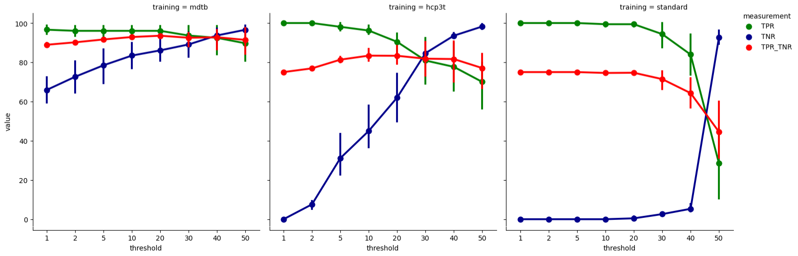
The summary measure of FIX accuracy (TPR_TNR; red curve) shows that dataset-specific training weights (mdtb) outperform both existing training weights (hcp3t and standard) at all thresholds. For the mdtb weights, the TPR (green curve) starts dropping off after 20, with relatively little TNR (blue curve) gained. The TPR_TNR summary measure also peaks at 20, indicating that this threshold strikes a good balance between high TPR and high TNR. Therefore, for cleaning the mdtb resting-state scans, we choose the mdtb trainingh weights as for component classification and apply a threshold of 20. For a more conservative cleanup, we would choose a lower threshold for high TPR and more signal retained, and for a more aggressive cleanup a higher threshold for high TNR but more signal removed.

Applying FIX

Now use the dataset-specific training weights to classify the components of each resting-state scan as signal and noise (or unkown) using the command /usr/local/fix/fix -c <Melodic-output.ica> mdtb.RData 20 with 20 as the chosen threshold. Once the labelling has finished, remove the variance that is unique to the noise components from each scan using /usr/local/fix/fix -a <mel.ica/fix4melview_mdtb_thr20.txt>. You can include the optional flag -m for removal of the full variance associated with the motion parameters preceding the noise component cleanup. And you can use the flag -A for aggressive noise cleanup (removes all noise variance, not just the unique variance). However, I leave both of those flags out, since in my experience full variance removal reduces cerebellar signal substantially (for example, removing the cerebellar node of the default network).

FIX will generate a cleaned fMRI data file called <original_name>_clean.nii.gz. Check that this was created once FIX has finished - and you’re done!

Addendum: Checking how FIX affected cerebellar correlations

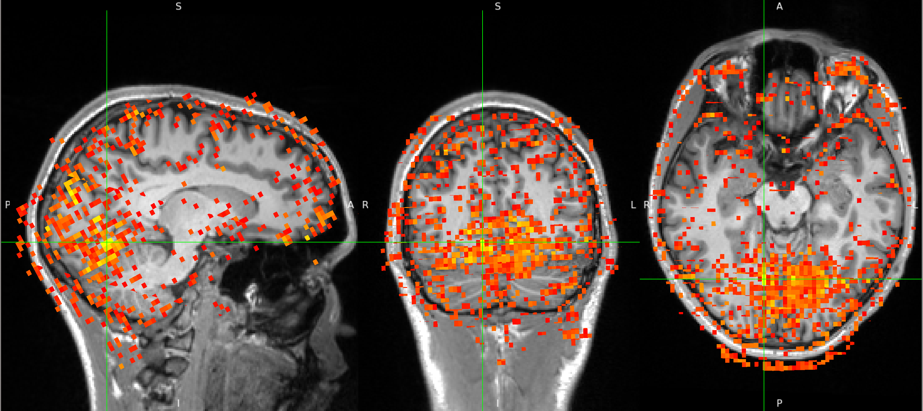
A big problem in cerebellar imaging is that non-neuronal noise (mostly due to physiological noise) can induce strong correlations between the fMRI timecourses of superior cerebellar voxels and voxels of the inferior occipital cortex. However, the visual cortex and the superior cerebellum are functionally not connected (no direct anatomical connections and no shared blood supply due to dura separating the two). Removing these spurious correlations from cerebellar data is tricky - making it an ideal test case for the FIX cleanup (credit goes to Joern Diedrichsen for the idea!).

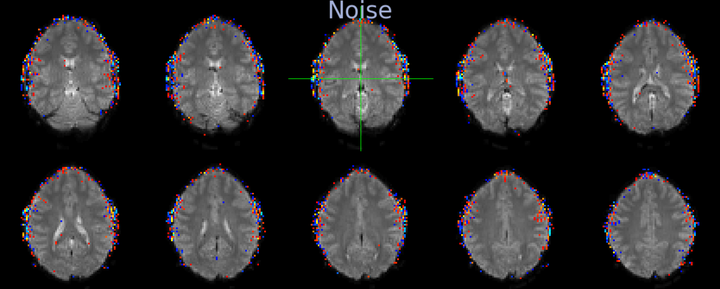
Below you can see a correlation map that results from extracting the timecourse from a seed voxel in the inferior occipital cortex and correlating it with the timecourses of all other voxels. The crosshair is placed at the seed location and the correlation values between 0.12 and 0.3 are shown. The map shows strong correlations across the occipital cortex - cerebellar boundary.

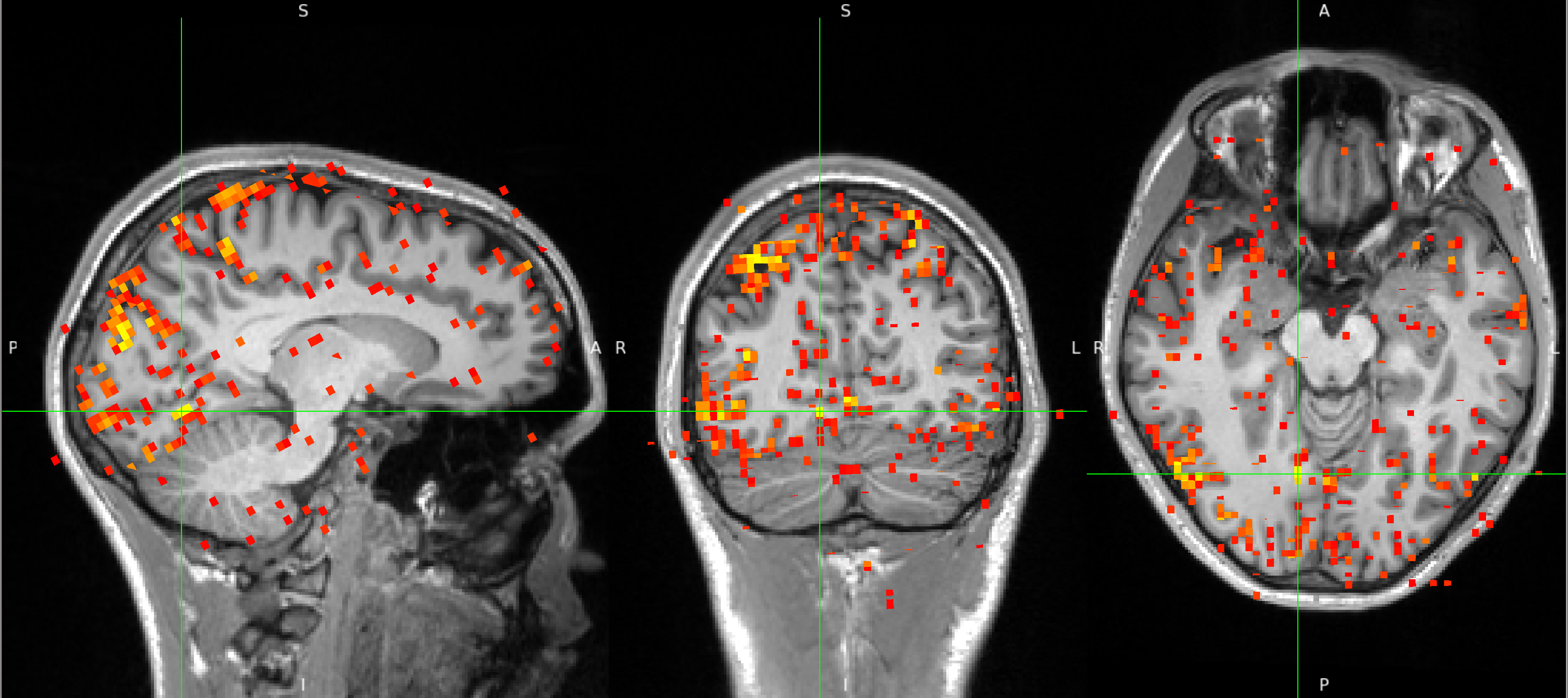
After FIX cleanup of the unique noise variance, the correlation map below shows barely any correlations between the inferior occipital cortex seed and the superior cerebellum. The map also shows far fewer correlations with voxels outside the brain, in CSF and white matter. Instead, the map shows primarily correlations with grey matter voxels that follow the gyri - a pattern that suggests primarily neuronal signal.

Links and Resouces

I picked up a lot that is covered here from excellent colleagues, including, but not limited to Ludo, Alberto, and the FSL Course Team. A special mention goes to Ludo’s fantastic teaching materials and papers on noise classification, which I have linked below:

Paper on Classifying Components: “ICA-based artefact removal and accelerated fMRI acquisition for improved resting state network imaging”

Educational course slides: “The Art and Pitfalls of fMRI Preprocessing”

FIX Classifier User Guide: Link

FEAT User Guide: Link